Notebook 4: Rational Method, Unit Hydrograph, Lumped & Distributed Models
Contents
Notebook 4: Rational Method, Unit Hydrograph, Lumped & Distributed Models#
Introduction to the unit hydrograph, the rational method, and lumped and distributed hydrological modelling.
Introduction#
In this notebook, we look at several ways of estimating a rainfall-runoff response hydrograph at varying levels of complexity.
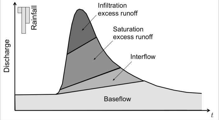
(source: Margulis 2020)
First, we’ll use the rational method to approximate peak flow for a small basin in the Whistler Village using empirical values. We’ll then introduce a few more complex models, including the Soil Conservation Service (SCS) models, the Unit Hydrograph (SCS-UH) and Curve Number (SCS-CN) models. We’ll calculate the peak runoff response using the CN method, where the basin properties like slope and roughness are assumed to be homogeneous across the basin. All areas of the basin in this case are treated as a single unit, often referred to as a “lumped” model.
Finally, we’ll use an open-source geospatial library to make a simple distributed model of the basin from digital elevation data (DEM). We’ll calculate the flow direction and flow accumulation in order to delineate a basin and define the stream network, and use this to construct an hydrograph from a precipitation event.
In all cases, we’ll relate the resulting flow to a practical problem involving water level in a hypothetical channel situated at the basin outlet. The purpose is to get a feel for the range of outcomes (the peak flow of the rainfall-runoff response hydrograph) under uncertain input variables.
# import required packages
import os
import pandas as pd
import numpy as np
# import math
# advanced statistics library
# from scipy import stats
import matplotlib.pyplot as plt
import matplotlib.patches as mp
import matplotlib.colors as colors
from pysheds.grid import Grid
working_directory = os.getcwd()
print(working_directory)
/home/danbot/Documents/UBC/CIVL_418_2022/Engineering_Hydrology_Notebooks/content/notebooks/Notebook_4
Find & Import Precipitation Data#
We can use the application from the Pacific Climate Impacts Consortium (PCIS) to retrieve climate observations in the Whistler area. For this exercise, we will use historical climate data from the Meteorological Service of Canada (MSC) station at Whistler, BC. Using the Observation Frequency filter provided, there appear to be a few climate stations with hourly precipitation data:
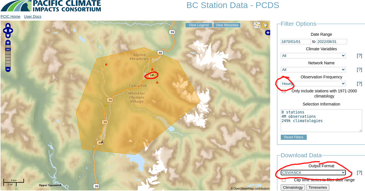
We’ll look at one (ID 1048899: Whistler (2014-2022)) as an example, but we’ll look at another as well because the PCIS web application suggests this station has hourly data but in fact it doesn’t, nor do any of the others except one (925 - green triangle circled in red). You are always responsible for your own data validation. In the
PCIS database has hourly data available at only one location in the Whistler area, and it’s from the Ministry of Forests, Lands, and Resource Operations Wildfire Management Branch (FLNRO-WMB) for a brief period in 2005 (ID 925 ZZ REMSATWX1).
# import precipitation data
daily_df = pd.read_csv('../../notebook_data/notebook_4_data/Whistler_348_climate.csv', parse_dates=True, index_col=['Date/Time'])
daily_df.dropna(subset=['Total Precip (mm)'], inplace=True)
daily_df.head()
| Station Name | Year | Month | Day | Data Quality | Max Temp (°C) | Max Temp Flag | Min Temp (°C) | Min Temp Flag | Mean Temp (°C) | ... | Total Snow (cm) | Total Snow Flag | Total Precip (mm) | Total Precip Flag | Snow on Grnd (cm) | Snow on Grnd Flag | Dir of Max Gust (10s deg) | Dir of Max Gust Flag | Spd of Max Gust (km/h) | Spd of Max Gust Flag | |
|---|---|---|---|---|---|---|---|---|---|---|---|---|---|---|---|---|---|---|---|---|---|
| Date/Time | |||||||||||||||||||||
| 1976-11-22 | WHISTLER | 1976 | 11 | 22 | NaN | 5.6 | NaN | NaN | M | NaN | ... | 0.0 | NaN | 1.5 | NaN | NaN | NaN | NaN | NaN | NaN | NaN |
| 1976-11-23 | WHISTLER | 1976 | 11 | 23 | NaN | 5.0 | NaN | 0.6 | NaN | 2.8 | ... | 0.0 | NaN | 12.7 | NaN | NaN | NaN | NaN | NaN | NaN | NaN |
| 1976-11-24 | WHISTLER | 1976 | 11 | 24 | NaN | 5.0 | NaN | 2.2 | NaN | 3.6 | ... | 0.0 | NaN | 2.5 | NaN | NaN | NaN | NaN | NaN | NaN | NaN |
| 1976-11-25 | WHISTLER | 1976 | 11 | 25 | NaN | 4.4 | NaN | 0.6 | NaN | 2.5 | ... | 0.0 | NaN | 0.0 | NaN | NaN | NaN | NaN | NaN | NaN | NaN |
| 1976-11-26 | WHISTLER | 1976 | 11 | 26 | NaN | 2.2 | NaN | -6.7 | NaN | -2.3 | ... | 0.0 | NaN | 0.0 | NaN | NaN | NaN | NaN | NaN | NaN | NaN |
5 rows × 27 columns
# note that the ascii file uses the string 'None' for NaN
# and we can deal with this on import.
hourly_df = pd.read_csv('../../notebook_data/notebook_4_data/925.ascii',
header=1, na_values=[' None'], infer_datetime_format=True, parse_dates=[' time'])
# note that the ascii format imports the column headers with spaces
# that need to be cleaned up
hourly_df.columns = [e.strip() for e in hourly_df.columns]
hourly_df.set_index('time', inplace=True, drop=True)
hourly_df.head()
| wind_speed | temperature | wind_direction | relative_humidity | precipitation | |
|---|---|---|---|---|---|
| time | |||||
| 2005-09-28 10:00:00 | 12.9 | 11.6 | 234.0 | 61.0 | 0.0 |
| 2005-09-28 11:00:00 | 14.8 | 11.2 | 229.0 | 68.0 | 0.0 |
| 2005-09-28 12:00:00 | 10.4 | 11.1 | 224.0 | 76.0 | 0.2 |
| 2005-09-28 13:00:00 | 13.8 | 10.5 | 247.0 | 79.0 | 0.0 |
| 2005-09-28 14:00:00 | 13.9 | 10.0 | 245.0 | 80.0 | 0.2 |
Plot the Data#
Here we will use the Bokeh data visualization library to plot the precipitation data. The ability to zoom in and out of different time scales provides a different perspective and helps with data exploration and review. We don’t have much data in this case, but if we did, holy crow, look out.
from bokeh.plotting import figure, show
from bokeh.io import output_notebook
from bokeh.models import ColorBar, ColumnDataSource
output_notebook()
hourly_source = ColumnDataSource(hourly_df)
daily_source = ColumnDataSource(daily_df)
p = figure(title=f'Precipitation', width=750, height=300, x_axis_type='datetime')
p.vbar(x='Date/Time', width=pd.Timedelta(days=1), top='Total Precip (mm)',
bottom=0, source=daily_source, legend_label='Daily Precipitation',
color='royalblue')
p.vbar(x='time', width=pd.Timedelta(hours=1), top='precipitation',
bottom=0, source=hourly_source, legend_label='Hourly Precipitation',
color='gold')
p.legend.location = 'top_left'
p.xaxis.axis_label = 'Date'
p.yaxis.axis_label = 'Precipitation [mm]'
p.toolbar_location='above'
show(p)
Use the zoom tool to compare the independent measurements over 28-29 September 2005. Do the daily volumes add up?
hourly_df['day'] = hourly_df.index.day
hourly_tot = hourly_df.groupby('day')['precipitation'].sum()
print(hourly_tot)
daily_check = daily_df['2005-09-28':'2005-09-29']['Total Precip (mm)'].copy()
print(daily_check)
day
28 17.4
29 22.8
Name: precipitation, dtype: float64
Date/Time
2005-09-28 26.2
2005-09-29 17.1
Name: Total Precip (mm), dtype: float64
The two day total is very close, but the volumes don’t line up despite these stations being in close proximity to each other (the Whistler station is the red triangle just north of the green triangle in the map above.)
If we happen to be interested in this particular day, what other information might be relevant as far as energy inputs? Take a look at the data columns:
daily_df.columns
Index(['Station Name', 'Year', 'Month', 'Day', 'Data Quality', 'Max Temp (°C)',
'Max Temp Flag', 'Min Temp (°C)', 'Min Temp Flag', 'Mean Temp (°C)',
'Mean Temp Flag', 'Heat Deg Days (°C)', 'Heat Deg Days Flag',
'Cool Deg Days (°C)', 'Cool Deg Days Flag', 'Total Rain (mm)',
'Total Rain Flag', 'Total Snow (cm)', 'Total Snow Flag',
'Total Precip (mm)', 'Total Precip Flag', 'Snow on Grnd (cm)',
'Snow on Grnd Flag', 'Dir of Max Gust (10s deg)',
'Dir of Max Gust Flag', 'Spd of Max Gust (km/h)',
'Spd of Max Gust Flag'],
dtype='object')
How about daily temperature and snow on the ground? How about data quality flags?
climate_check = daily_df['2005-09-28':'2005-09-29'][['Snow on Grnd (cm)', 'Mean Temp (°C)']].copy()
climate_check
| Snow on Grnd (cm) | Mean Temp (°C) | |
|---|---|---|
| Date/Time | ||
| 2005-09-28 | 0.0 | 7.0 |
| 2005-09-29 | 0.0 | 10.1 |
flag_check = daily_df['2005-09-28':'2005-09-29'][['Snow on Grnd Flag', 'Mean Temp Flag', 'Total Precip Flag']].copy()
flag_check
| Snow on Grnd Flag | Mean Temp Flag | Total Precip Flag | |
|---|---|---|---|
| Date/Time | |||
| 2005-09-28 | NaN | NaN | NaN |
| 2005-09-29 | NaN | NaN | NaN |
No data flags, and no snow on the ground, so we might have a bit more confidence in the daily data, although it’s difficult to reconcile the timing between the two sets. It could be a timezone issue, i.e. some agencies report times in UTC which is 7-8 hours ahead, or it could be a matter of how the timestamps are handled when data is aggregated.
Problem Setup#
Let’s imagine you had a summer job in Whistler working on a project to grade and re-pave the area around Day Lot 4, including installing drainage to capture water from the parking lot and divert it to a storm water collection system instead of draining into FitzSimmons Creek. We are in charge of constructing a temporary diversion channel to redirect water from the project area so it doesn’t run directly into Fitzsimmons Creek and risk damaging the aquatic ecosystem.
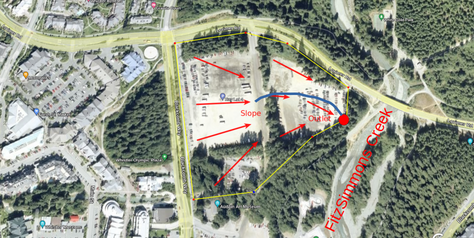
It’s summer and the project is scheduled to be completed by fall. For the sake of this exercise, assume the slope of the parking lot area describes a catchment of roughly 1 \(km^2\) and empties through a temporary channel into a catch basin to be treated before flowing into FitzSimmons Creek.
Note: Given the drainage area is only \(1 km^2\), do you have a sense of what duration of rainfall is appropriate for estimating the peak of the runoff response hydrograph? i.e. 1 minute, 10 minutes, 1h, 6h, 24h, 48h?
There appears to be a spot that could be a natural outlet channel which would avoid excavation and accelerate the project schedule, so you go out and survey the location to get accurate dimensions. Assume this natural channel has the following geometry.
Channel width (w): \(3m\)
Channel Depth (h): \(0.5m\)
Hydraulic Grade Line Slope (S): 0.005 (0.5%)
Roughness (n): 0.017 (rough asphalt)
Calculate the channel capacity#
Since the dimensions are known it’s much easier to determine its capacity. We’ll calculate the capacity first and then see how our estimates of peak runoff compare. Open channel flow is given by the Manning equation:
w, h = 2, 0.5 # height, width in metres
# cross section area
A = w * h
perim = 2 * w + 2 * h
# hydraulic radius
R = A / perim
# streamwise slope
S = 0.005
# roughness coefficient
n_manning = 0.017
# average velocity
V_avg_open_channel = R**(2.0/3) * S**(1.0/2) / n_manning
print(f'The average channel velocity for full capacity flow is {V_avg_open_channel:.1f}m/s')
Q_channel_capacity = V_avg_open_channel * A
print(f'The capacity of the channel is {Q_channel_capacity:.1f} m^3/s')
The average channel velocity for full capacity flow is 1.4m/s
The capacity of the channel is 1.4 m^3/s
Hydrograph Estimation#
It is rare to find long-term records at a high frequency of measurement, so we do the best we can with the information available. Below, we’ll look at a few ways of constructing a hydrograph of varying amounts of detail. We want to construct a hydrograph, or at least accurately predict its peak, in order to design hydraulic structures and other water management systems. We’ll start with a very basic estimate that has minimal information requirements, and move to more complex and information-intensive methods.
Water resources problems are often expressed in terms of risk, and typically for this kind of analysis we communicate risk in terms of annual exceedance probability (AEP). In other words, what is the probability that the flow passing some location will exceed the channel (or built structure) capacity in a given year? These kinds of problems do not have a right answer, they are open-ended and subjective—meaning any answer involves some amount of (engineering) judgment. The topic of risk will be discussed further in Notebook 5. For now, we’ll just focus on a few ways of estimating a runoff hydrograph from precipitation data.
Convert volume (mm or in per hour or day) to volumetric flow units#
Runoff is typically measured in \(\frac{m^3}{s}\), and precipitation is often reported in mm or in per hour or day. Convert \(\frac{mm}{day}\) precipitation to \(\frac{m^3}{s}\).
Rational Method#
Recall that the peak runoff for a small basin can be estimated by the following from the US Army Corps of Engineers (USACE):
Where:
Q: is the peak discharge of the event [\(m^3/s\)]
k: 0.278 [-] Note: \(\quad 1\frac{mm}{hr} \cdot \frac{1\text{hr}}{3600s} \cdot \frac{1m}{1000mm} \cdot 1 \text{km}^2 \cdot \frac{1\times 10^6 m^2}{1\text{km}^2} = \frac{1}{3.6} = 0.278 \frac{m^3}{s}\)
C: runoff coefficient [-]
I: rainfall intensity [mm/hr]
a: drainage area [\(km^2\)]
We have already estimated drainage area, and there are just two additional pieces of information we need to estimate the peak runoff for our basin. The ratio of runoff to precipitation (the runoff coefficient) “C” can be found in a table of empirical values in the USACE link above, and the rainfall intensity can be estimated from Intensity-Duration-Frequency curve data developed by Environment Canada. More information on IDF Curve usage can be found here. We can find IDF curves for specific locations using the web application at climatedata.ca. The IDF curve for Whistler is below:
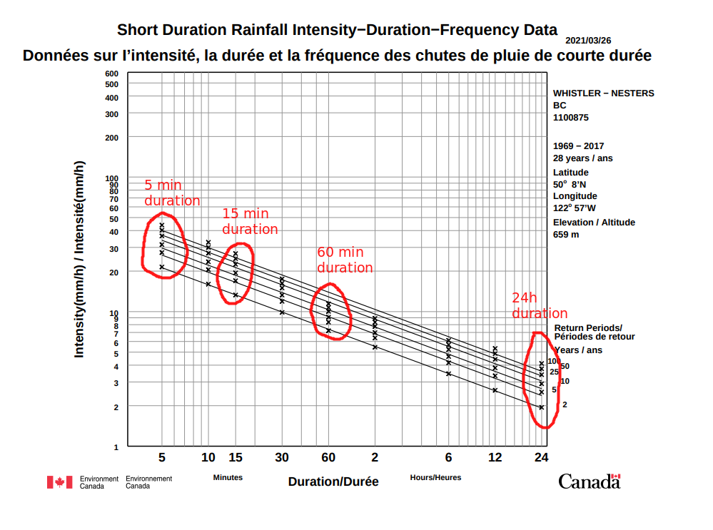
We don’t really know the appropriate duration (x-axis) yet for our basin, but we can select a few and run calculations to see how sensitive this model is to the duration. The five diagonal lines represent different return periods (2, 5, 10, 20, 50, 100 years). The return period is the inverse of the AEP, and again it represents the probability of occurrence in any given year, and it does not suggest an event of any magnitude will occur once in that return period.
Below we’ll express the values that we’re not too sure about as plausible ranges, and test their effect on the result.
def rational_method_peak_flow(C, I, a):
"""Calculate peak flow (in) using the rational method.
Args:
C (float): runoff coefficient [-]
I (float): rainfall intensity [mm/hr]
a (float): drainage area [km^2]
"""
return C * I * a / 3.6
# for each return period, we'll read the minimum and maximum intensity
# and use these to see the range of outcomes
# duration (minutes): volume (mm)
IDF_dict = {
5: (22, 45), # the 2 and 100 year intensities are 22mm, 45mm / h
15: (14, 28),
60: (7, 15),
1440: (2, 4) # 1440 minutes is 24 hours
}
# here we'll define an array of three runoff coefficient values
# to get a sense of the range of possible conditions
# minimum, maximum, and expected value
C_values = [0.5, 0.7, 0.9]
# calculate the range of flow estimates for each C and each return period
# and create a plot for each runoff coefficient
figs = []
rational_results = {}
colors=['green', 'orange', 'red']
for k, (i_min, i_max) in IDF_dict.items():
i = 0
p = figure(title=f'Duration={k}min', width=600, height=400)
for c in C_values:
Q_min = rational_method_peak_flow(c, i_min, 1)
Q_max = rational_method_peak_flow(c, i_max, 1)
print(f'{k} minutes duration, C={c} Q_range = {Q_min:.1f} to {Q_max:.1f} cms')
x = [2, 100]
y = [Q_min, Q_max]
p.line(x, y, legend_label=f'C={c}', color=colors[i])
p.yaxis.axis_label = 'Flow [m^3/s]'
p.xaxis.axis_label = 'Return Period'
p.legend.location = 'top_left'
i += 1
figs.append(p)
5 minutes duration, C=0.5 Q_range = 3.1 to 6.2 cms
5 minutes duration, C=0.7 Q_range = 4.3 to 8.7 cms
5 minutes duration, C=0.9 Q_range = 5.5 to 11.2 cms
15 minutes duration, C=0.5 Q_range = 1.9 to 3.9 cms
15 minutes duration, C=0.7 Q_range = 2.7 to 5.4 cms
15 minutes duration, C=0.9 Q_range = 3.5 to 7.0 cms
60 minutes duration, C=0.5 Q_range = 1.0 to 2.1 cms
60 minutes duration, C=0.7 Q_range = 1.4 to 2.9 cms
60 minutes duration, C=0.9 Q_range = 1.8 to 3.8 cms
1440 minutes duration, C=0.5 Q_range = 0.3 to 0.6 cms
1440 minutes duration, C=0.7 Q_range = 0.4 to 0.8 cms
1440 minutes duration, C=0.9 Q_range = 0.5 to 1.0 cms
from bokeh.layouts import gridplot
layout = gridplot(figs, ncols=2, width=350, height=300)
show(layout)
Pause and reflect: From the plots above, is it more important to get the correct duration, to select an appropriate return period, or to get an accurate estimate of the runoff coefficient? In other words, how sensitive is the model to the different input parameters?
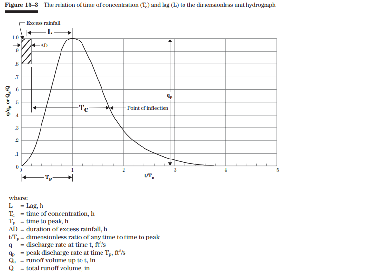
SCS Unit Hydrograph Model#
The unit hydrograph diagram below describes an idealized basin response to precipitation, and it is used in physically-based models to estimate the peak of the hydrograph response. The shape of the hydrograph has many influences, and it is controlled by complex interactions between the atmosphere, the surface (i.e. vegetation, roughness, slope), and the subsurface (i.e. antecedent soil moisture, permeability, porosity). Generally these values are carefully calibrated by concurrent runoff and precipitation measurement covering the broadest possible range of conditions.
The information requirement is intensive for the SCS-UH method compared to the rational method, and it is highly dependent upon a specific location and highly variable in time. This information may be available in some applications like urban hydrology where detailed survey information, surfaces, slopes, etc. can be acquired. In such a case the Soil Conservation Service (SCS) Unit Hydrograph model may be useful.
\(U_P\): peak flow
\(C\): conversion constant
\(A\): basin area
\(T_p\): time of peak
(source: USDA National Engineering Handbook: Chapter 15 - Time of Concentration)
A more intuitive description of time of concentration \(t_c\) is the time it takes for flow to travel from the furthest point in the watershed to the outlet. The \(t_c\) approximate the furthest flow path in our basin and break it up into components:
The above three flow components are just a 3-parameter model of the average velocity of flow over the longest flow path. In reality, we should use only as many parameters as we can defend with evidence. Again, these estimates should in reality be based on careful field observation. For our simple example problem, we won’t elaborate further than showing the equations for estimating times.
Where:
\(N\): overland roughness coefficient [-]
\(L\): length of flow path [ft]
\(P\): 2-year 24h rainfall depth rainfall depth [in]
\(S\): slope of hydraulic grade line (land slope) [ft/ft]
\(V\): average (shallow flow) velocity [ft/s]
From Figure 3-1 of SCS Curve Number Method documentation, we can estimate the average flow velocity for shallow concentrated flow over unpaved surface (gravel) is 1.2 ft/s (0.37 m/s). For a 250m channel length this translates to 0.2 hours. We can use this to estimate the time of concentration for our basin.
Note: Careful with units here! Lots of older technical documentation is written in imperial units (ft-lb) and we need to be sure that empirical coefficients are not introducing errors in our calculations.
def calculate_t_sheet(n, L, P, s):
"""
n: dimensionless surface roughness [-]
s: slope (ft/ft)
L: flow path length (ft)
P:
"""
return 0.007 * (n * L)**0.8 / ((P**0.5) * s**0.4 )
t_t = 0.2 # 0.2 hour channel flow
n = 0.0011
s = 0.005
L = 330 # 100m is roughly 300 ft.
# From IDF curve, 2-year 24h volume is 2mm/h * 24h = 48mm = ~1.9 inches
P_in = 1.9
t_sheet = calculate_t_sheet(n, L, P_in, s)
print(f'Time of concentration is approximately {t_sheet+t_t:.2f} hours: {t_sheet:.2f}hr (sheet) + {t_t:.2f} (shallow).')
Time of concentration is approximately 0.22 hours: 0.02hr (sheet) + 0.20 (shallow).
Above, we estimated the time of concentration for this very small basin which should help reduce the range of peak flow estimates calculated above, where we assumed a range of 5 minutes to 24 hours duration to get our values for intensity. We might be justified in narrowing our range between 10 and 30 minutes or so if we are confident in the time of concentration estimate.
SCS Curve Number (CN) Method#
The SCS Curve Number Method requires less information but has a few more parameters compared to the rational method to approximate surface losses by classifying the land cover (see Chapter 2 in the linked pdf):
\(P\): rainfall volume [in/[time]]
\(S\): potential retention after runoff begins [in]
\(I_a\): initial losses before runoff begins [in] (\(I_a \approx 0.2S\))
CN: curve number (from below)
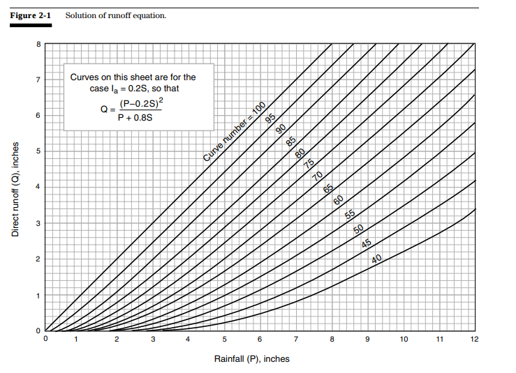
From Table 2-2a in the CN method document, curve numbers for gravel roads range from 76 to 91 for hydrologic soil groups A, B, C, and D.
We also need to estimate the time of concentration, which is discussed in Chapter 3 of the SCS CN method document linked above. We’ve already developed an estimate of time of concentration above.
def CN_method_Q(p_mm, cn):
"""Calculate peak Q (m^3/s) from the curve number.
CN is the curve number corresponding to soil type.
S is a factor related to retention (storage) after runoff begins.
P is a rainfall volume.
"""
S = (1000.0 / cn) - 10
p_in = p_mm / 25.4 # convert to inches
V_in = (p_in - 0.2 * S)**2 / (p_in + 0.8 * S) # in/h
# 1 inch = 25.4 mm
V_mm = V_in * 25.4 # mm/hr
# convert mm volume to m^3/s for 1 km^2
V_cms = (V_mm / 3600) * (1E6 / 1000)
return V_cms
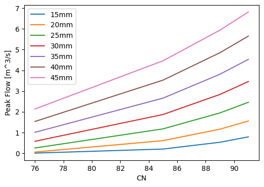
CNs = [76, 85, 89, 91]
# precip values are estimated as a range
# from the IDF curves above for 15 min and 60 min
# duration for 2 to 100 year return period intensity
p_estimates_mm = [12, 15, 28] # mm/h
p_range = list(range(15, 50, 5))
CN_Q = {}
for p in p_range:
CN_Q[p] = []
for cn in CNs:
V_cms = CN_method_Q(p, cn)
CN_Q[p].append(V_cms)
Plot the results of the CN Method#
cn_df = pd.DataFrame(CN_Q)
fig, ax = plt.subplots(figsize=(6, 4))
for p in p_range:
ax.plot(CNs, cn_df[p], label=f'{p}mm')
ax.set_xlabel('CN')
ax.set_ylabel('Peak Flow [m^3/s]')
ax.legend()
<matplotlib.legend.Legend at 0x7ff0d5350c10>
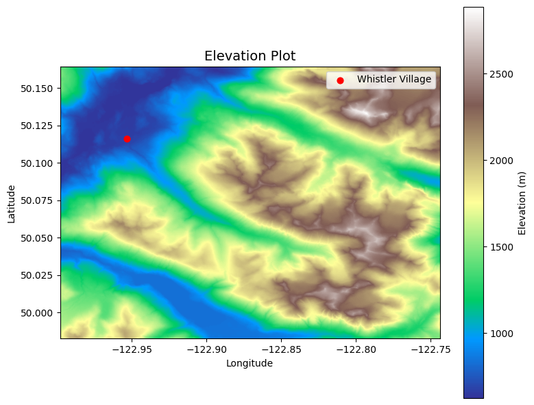
Distributed Model from Spatial Data#
As discussed in class, precipitation takes time to flow to the basin outlet, and there are complex interactions with the atmosphere, vegetation, the ground surface, and the subsurface that make predicting the basin response to precipitation very difficult to model accurately. Now we’ll use DEM data to delineate a basin and make a simple distributed model to create a unit hydrograph from hourly and daily precipitation data, and attempt to compare the volume of runoff predicted by our model against a value measured in Fitzsimmons Creek.
Note: From here we leave the example 1 \(\text{km}^2\) basin example and look at a larger basin in the same area but draining Fitzsimmons Creek.
Import the DEM and plot the data#
Here we’ll use the Pysheds library to process the DEM.
data_path = '../../notebook_data/notebook_4_data/'
dem_file = 'Whistler_DEM.tif'
dem_path = data_path + dem_file
grid = Grid.from_raster(dem_path)
dem = grid.read_raster(dem_path)
fig, ax = plt.subplots(figsize=(8,6))
fig.patch.set_alpha(0)
plt.imshow(dem, extent=grid.extent, cmap='terrain', zorder=2)
plt.colorbar(label='Elevation (m)')
# show whistler on the DEM
plt.scatter(x=[-122.9535], y=[50.1162], zorder=3, c='red', s=40, label='Whistler Village')
plt.grid(zorder=0)
plt.title('Elevation Plot', size=14)
plt.xlabel('Longitude')
plt.ylabel('Latitude')
plt.legend()
plt.tight_layout()
Fill Pits and Resolve flats in DEM#
The sampling of surface elevations from a DEM often contain depressions and flat regions that must be filled in order for flow accumulation networks (streams) to resolve.
# Condition DEM
# ----------------------
# Fill pits in DEM
pit_filled_dem = grid.fill_pits(dem)
# Fill depressions in DEM
flooded_dem = grid.fill_depressions(pit_filled_dem)
# Resolve flats in DEM
inflated_dem = grid.resolve_flats(flooded_dem)
Derive flow directions from DEM#
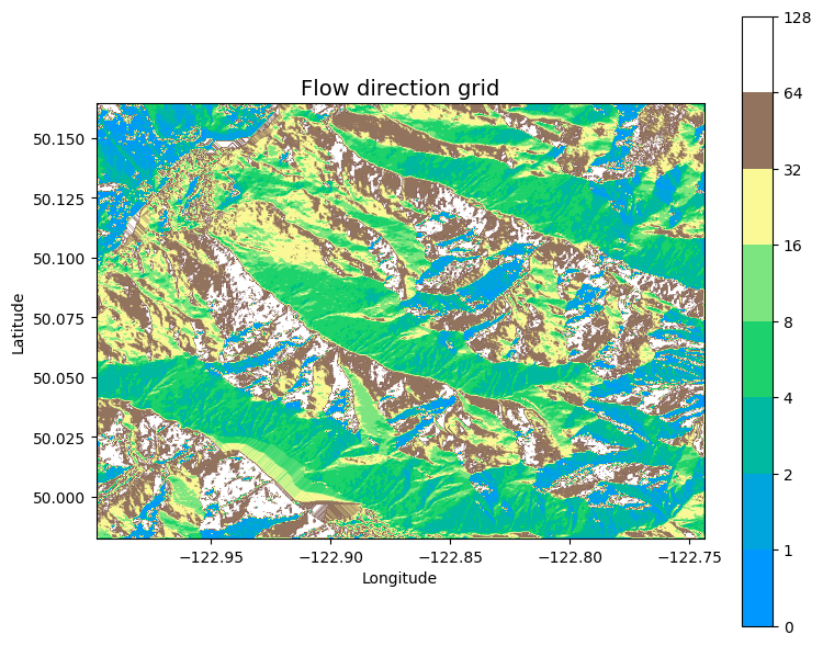
Each cell of a DEM raster is assigned a flow direction calculated by determining the slope at that pixel/cell. The slope is determined by comparing elevations with the 8 surrounding/connected pixels. Directions are assigned one of eight values corresponding to 8-bit integers (\(2^1, 2^2, 2^3, \dots 2^7\))
32 |
64 |
128 |
16 |
- |
1 |
8 |
4 |
2 |
import matplotlib.cm as cmx
import matplotlib.colors as colors
# Determine D8 flow directions from DEM
# ----------------------
# Specify directional mapping
dirmap = (64, 128, 1, 2, 4, 8, 16, 32)
# Compute flow directions
# -------------------------------------
fdir = grid.flowdir(inflated_dem, dirmap=dirmap)
fig = plt.figure(figsize=(8,6))
fig.patch.set_alpha(0)
# we have to normalize the colors to provide contrast
cNorm = colors.PowerNorm(gamma=0.5)
plt.imshow(fdir, extent=grid.extent, norm=cNorm,
cmap='terrain', zorder=2)
boundaries = ([0] + sorted(list(dirmap)))
plt.colorbar(boundaries= boundaries,
values=sorted(dirmap))
plt.xlabel('Longitude')
plt.ylabel('Latitude')
plt.title('Flow direction grid', size=14)
plt.grid(zorder=-1)
plt.tight_layout()
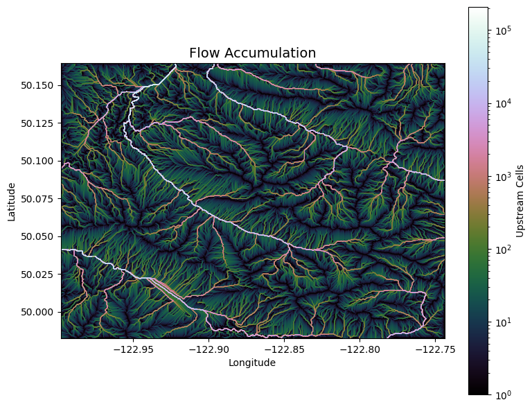
Get flow accumulation#
Recall from the exercise in class how we derived flow accumulation from the flow direction. Each cell has a direction associated with it. Flow accumulation in this case is expressed as the number of upstream cells.
# Calculate flow accumulation
# --------------------------
acc = grid.accumulation(fdir, dirmap=dirmap)
fig, ax = plt.subplots(figsize=(8,6))
fig.patch.set_alpha(0)
plt.grid('on', zorder=0)
im = ax.imshow(acc, extent=grid.extent, zorder=2,
cmap='cubehelix',
norm=colors.LogNorm(1, acc.max()),
interpolation='bilinear')
plt.colorbar(im, ax=ax, label='Upstream Cells')
plt.title('Flow Accumulation', size=14)
plt.xlabel('Longitude')
plt.ylabel('Latitude')
plt.tight_layout()
Delineate a Catchment#
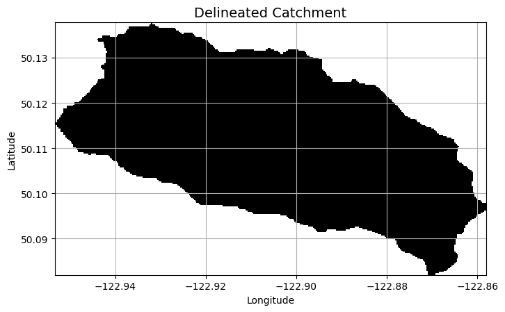
Below we will delineate a basin corresponding to the hydrometric station located on Fitzsimmons Creek. Water Survey of Canada have recently published basin polygons for nearly 7000 stations across Canada. In addition, pour points are also provided as shape files. A limitation of Whiteboxtools is we need to specify the pour point as a file (.shp or .geojson) and we can’t just provide coordinates. The pour point is the outlet of the basin. If we have high resolutoin data and imperfect coordinates of a pour point, we will not get the correct pixel corresponding to the outlet.
# Delineate a catchment
# ---------------------
# Specify pour point (WSC Station at Fitzsimmons Creek in Whistler: 08MG026)
x, y = -122.9488, 50.12025
# specify a threshold for flow accumulation in cells
# for this raster, 500 cells is roughly 0.5 km^2
accumulation_threshold = 500
# Snap pour point to high accumulation cell
x_snap, y_snap = grid.snap_to_mask(acc > 1000, (x, y))
# Delineate the catchment
catch = grid.catchment(x=x_snap, y=y_snap, fdir=fdir, dirmap=dirmap,
xytype='coordinate')
# Crop and plot the catchment
# ---------------------------
# Clip the bounding box to the catchment
grid.clip_to(catch)
clipped_catch = grid.view(catch)
# Plot the catchment
fig, ax = plt.subplots(figsize=(8,6))
fig.patch.set_alpha(0)
plt.grid('on', zorder=0)
im = ax.imshow(np.where(clipped_catch, clipped_catch, np.nan), extent=grid.extent, zorder=1, cmap='Greys_r')
plt.xlabel('Longitude')
plt.ylabel('Latitude')
plt.title('Delineated Catchment', size=14)
Text(0.5, 1.0, 'Delineated Catchment')
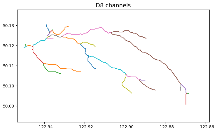
# Extract river network
# ---------------------
branches = grid.extract_river_network(fdir, acc > 500, dirmap=dirmap)
fig, ax = plt.subplots(figsize=(8.5,6.5))
plt.xlim(grid.bbox[0], grid.bbox[2])
plt.ylim(grid.bbox[1], grid.bbox[3])
ax.set_aspect('equal')
for branch in branches['features']:
line = np.asarray(branch['geometry']['coordinates'])
plt.plot(line[:, 0], line[:, 1])
_ = plt.title('D8 channels', size=14)
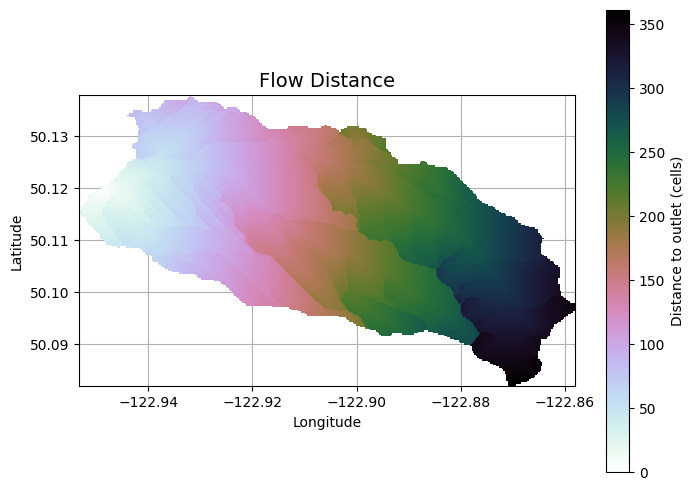
Calculate distances to upstream cells#
# Calculate distance to outlet from each cell
# -------------------------------------------
dist = grid.distance_to_outlet(x=x_snap, y=y_snap, fdir=fdir, dirmap=dirmap,
xytype='coordinate')
fig, ax = plt.subplots(figsize=(8,6))
fig.patch.set_alpha(0)
plt.grid('on', zorder=0)
im = ax.imshow(dist, extent=grid.extent, zorder=2,
cmap='cubehelix_r')
plt.colorbar(im, ax=ax, label='Distance to outlet (cells)')
plt.xlabel('Longitude')
plt.ylabel('Latitude')
plt.title('Flow Distance', size=14)
Text(0.5, 1.0, 'Flow Distance')
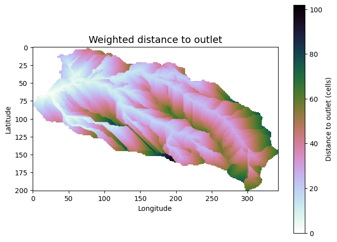
Calculate weighted travel distance#
Assign a travel time to each cell based on the assumption that water travels at one speed (overland flow is slower) until it accumulates into a stream network, at which point its speed increases dramatically.
# Compute flow accumulation
acc = grid.accumulation(fdir)
# Assume that water in channelized cells (>= 500 accumulation)
# travels 10 times faster than hillslope cells (< 500 accumulation)
# i.e. if average channel velocity is 1m/s, hillslope is 0.1m/s = 10 cm/s
weights = acc.copy()
weights[acc >= accumulation_threshold] = 0.1
weights[(acc > 0) & (acc < accumulation_threshold)] = 1
# # Compute weighted distance to outlet
weighted_dist = grid.distance_to_outlet(x=x_snap, y=y_snap, fdir=fdir, weights=weights, xytype='coordinate')
fig, ax = plt.subplots(figsize=(8,6))
fig.patch.set_alpha(0)
# plt.grid('on', zorder=0)
im = ax.imshow(weighted_dist, zorder=2,
cmap='cubehelix_r')
plt.colorbar(im, ax=ax, label='Distance to outlet (cells)')
plt.xlabel('Longitude')
plt.ylabel('Latitude')
plt.title('Weighted distance to outlet', size=14)
Text(0.5, 1.0, 'Weighted distance to outlet')
Develop a simple rainfall-runoff model#
Now that we have weighted flow distances for each cell in the delineated catchment, we can apply precipitation to each ‘cell’ in order to reconstruct a flow hydrograph.
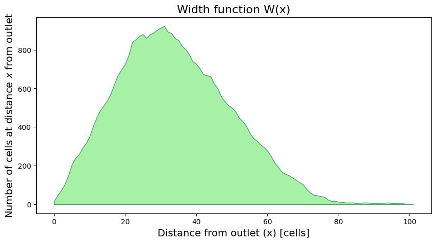
First, we need the cell dimensions (the size of each raster pixel on the ground). From the USGS Hydrosheds information, we know the resolution is 15 (degree) seconds. Because the earth is not a perfect sphere, coordinate projection systems (CRS) are used to approximate the surface of the earth so that spatial distances can be more accurately represented.
Note that our ‘weighted distance’ has just provided a relative difference between the flow accumulation cells and non-flow-accumulation cells. We still must convert these values to some time-dependent form.
For this exercise, we will assume the average velocity of water is 1 m/s value for the flow accumulation cells, and 0.01 m/s for hillslope cells. Let’s calculate the unweighted and weighted time of concentration (time to travel from furthest cell to the outlet).
The DEM is from the USGS 3DEP program and is roughly 30m resolution (each pixel represents a square area of roughly 30m by 30m). We have reduced the (distance) weight of channel cells, so the distance is proportional to our estimate of hillslope velocity, and we can convert the distance to time by dividing the weighted distance by 1 m/s.
# get the raster pixel resolution (m by m)
resolution = (30, 30)
# cells can be grouped by their weighted distance to the outlet to simplify
# the process of calculating the contribution of each cell to flow at the outlet
dist_df = pd.DataFrame()
dist_df['weighted_dist'] = weighted_dist.flatten()
# trim the distance dataframe to include only the cells in the catchment,
# and round the travel time to the nearest distance unit (number of cells)
dist_df = dist_df[np.isfinite(dist_df['weighted_dist'])].round(0)
# get the number of cells of each distance
grouped_dists = pd.DataFrame(dist_df.groupby('weighted_dist').size())
grouped_dists.columns = ['num_cells']
# plot distributions of weighted distance
W = np.bincount(weighted_dist[np.isfinite(weighted_dist)].astype(int))
fig, ax = plt.subplots(figsize=(10, 5))
plt.fill_between(np.arange(len(W)), W, 0, edgecolor='seagreen', linewidth=1, facecolor='lightgreen', alpha=0.8)
plt.ylabel(r'Number of cells at distance $x$ from outlet', size=14)
plt.xlabel(r'Distance from outlet (x) [cells]', size=14)
plt.title('Width function W(x)', size=16)
Text(0.5, 1.0, 'Width function W(x)')
flow_velocity = 0.1 # m/s
w_time = weighted_dist * resolution[0] / flow_velocity / 3600
W_time = np.bincount(w_time[np.isfinite(w_time)].astype(int))
fig, ax = plt.subplots(figsize=(10, 5))
plt.fill_between(np.arange(len(W_time)), W_time, 0, edgecolor='seagreen', linewidth=1, facecolor='lightgreen', alpha=0.8)
plt.ylabel(r'Number of cells $x$ hours from outlet', size=14)
plt.xlabel(r'Time to outlet $x$ (hours)', size=14)
plt.title('Width function W(x) ~ Unit Hydrograph', size=16)
Text(0.5, 1.0, 'Width function W(x) ~ Unit Hydrograph')
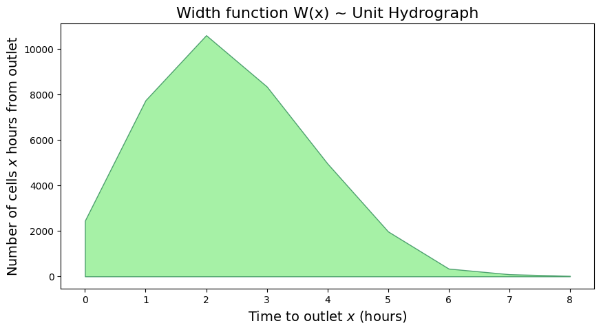
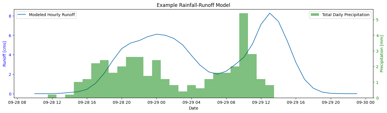
Note: Above we’ve developed an estimated unit hydrograph for 1 unit of precipitation falling uniformly over the basin, and we did it with just elevation data and an estimate of the difference in flow velocities between stream and slope flow.
Calculate total runoff and compare against measured daily volume for the two day record#
NOTE: if you update the runoff coefficient below, you must re-run the code from here to re-initialize the
runoff_dfdataframe, otherwise the values will accumulate.
# create unit hydrographs for each timestep
runoff_df = pd.DataFrame(np.zeros(len(hourly_df)))
runoff_df.columns = ['Total Precip (mm)']
runoff_df.index = hourly_df.index.copy()
end_date = pd.to_datetime(runoff_df.index.values[-1]) + pd.DateOffset(hours=1)
max_distance = max(grouped_dists.index)
def calculate_flow_time(distance, v):
# convert flow path length (in cells)
# to a travel time
return np.ceil(distance * resolution[0] / v / 3600)
# time of concentration
max_flow_time = calculate_flow_time(max_distance, flow_velocity)
print(f'The maximum adjusted flow path is {max_distance} cells, corresponding to a maximum flow travel time of {max_flow_time} hours.')
extended_df = pd.DataFrame()
extended_df['Total Precip (mm)'] = [0 for e in range(int(max_flow_time) + 1)]
extended_df.index = pd.date_range(end_date, periods=max_flow_time + 1, freq='1H')
# append the extra time to the runoff dataframe
runoff_df = pd.concat([runoff_df, extended_df])
runoff_df['Runoff (cms)'] = 0
The maximum adjusted flow path is 102.0 cells, corresponding to a maximum flow travel time of 9.0 hours.
The cell below is a big computation and may take some time. What is happening below is for each hour of precipitation, we calculate the time offset for the flow to get from each cell to the outlet. Each cell does not take the same amount of time for flow to get to the outlet, so we add each cell’s runoff at the future time corresponding to the cell’s travel time. We make it slightly more efficient by grouping cells of equal distance.
Below we estimate a runoff coefficient of 0.3, in other words 30% of our precipitation will be excess. Later we’ll see how the model results compare to measured values and try to validate this coefficient.
runoff_coefficient = 0.3
for ind, row in hourly_df.iterrows():
this_hyd = hourly_df[['precipitation']].copy()
hydrograph = pd.DataFrame()
for weight_dist, num_cells in grouped_dists.iterrows():
weighted_time = calculate_flow_time(weight_dist, flow_velocity)
outlet_time = ind + pd.Timedelta(hours=weighted_time)
# round the travel time to nearest hour
# to align with hourly streamflow data
if weighted_time < 1:
outlet_time = ind + pd.Timedelta(hours=1)
precip_vol = num_cells.values[0] * row['precipitation']
runoff_vol = precip_vol * runoff_coefficient / 1000 * resolution[0]**2
runoff_rate = runoff_vol / 3600 # convert to m^3/s from m^3/h
runoff_df.loc[outlet_time, 'Runoff (cms)'] += runoff_rate
runoff_df['day'] = runoff_df.index.day
# convert m^3/s to m^3/hour (cmh)
runoff_df['runoff_vol_cmh'] = runoff_df['Runoff (cms)'] * 3600
cumulative_vol = runoff_df[['runoff_vol_cmh', 'day']].groupby('day').sum()
cumulative_vol
| runoff_vol_cmh | |
|---|---|
| day | |
| 28 | 102690.396 |
| 29 | 293762.808 |
# import runoff time series
whis_flow_df = pd.read_csv(os.path.join(data_path, '08MG026_daily.csv'),
header=1, parse_dates=['Date'], index_col=['Date'])
# whis_flow_df = whis_flow_df[whis_flow_df['2005-09-27': '2005-09-31']]
# whis_flow_df
whis_flow_df = whis_flow_df['2005-09-27':'2005-09-30'].round(1)
whis_flow_df
| ID | PARAM | Value | SYM | |
|---|---|---|---|---|
| Date | ||||
| 2005-09-27 | 08MG026 | 1 | 1.3 | NaN |
| 2005-09-28 | 08MG026 | 1 | 1.5 | NaN |
| 2005-09-29 | 08MG026 | 1 | 4.8 | NaN |
| 2005-09-30 | 08MG026 | 1 | 2.8 | NaN |
cumulative_vol.values.flatten()
whis_flow_df.loc['2005-09-28':'2005-09-29']
| ID | PARAM | Value | SYM | |
|---|---|---|---|---|
| Date | ||||
| 2005-09-28 | 08MG026 | 1 | 1.5 | NaN |
| 2005-09-29 | 08MG026 | 1 | 4.8 | NaN |
# for the whistler runoff, subtract the base flow
# assume this is 1.3 cms from Sept. 27th
whis_flow_df['excess_flow'] = whis_flow_df['Value'] - 1.3
# convert daily average flow to daily volume in m^3/day
whis_flow_df['excess_volume'] = whis_flow_df['excess_flow'] * 3600 * 24
whis_flow_df.loc['2005-09-28':'2005-09-29', 'model_volume'] = cumulative_vol.values.flatten()
fig, ax = plt.subplots(1, 1, figsize=(16,4))
ax.plot(runoff_df.index, runoff_df['Runoff (cms)'], label="Modeled Hourly Runoff")
# ax.plot(whis_flow_df.index, whis_flow_df['Value'], label='Measured Daily Avg. [m^3/s]')
ax.set_xlabel('Date')
ax.set_ylabel('Runoff [cms]', color='blue')
ax.set_title('Example Rainfall-Runoff Model')
ax.legend(loc='upper left')
ax.tick_params(axis='y', colors='blue')
ax1 = ax.twinx()
# plot the precipitation
ax1.bar(hourly_df.index, width=pd.Timedelta(hours=1),
height=hourly_df['precipitation'], color='green', alpha=0.5,
label="Total Daily Precipitation")
ax1.set_ylabel('Precipitation [mm]', color='green')
ax1.tick_params(axis='y', colors='green')
ax1.legend(loc='upper right')
<matplotlib.legend.Legend at 0x7ff0d7030580>
Compare the modeled and measured runoff#
We can’t directly compare hourly modeled and daily measured flow, but we can compare the total volume. Compare the modeled excess runoff from precipitation vs. the measured runoff (adjusted for base flow). Below we subtract the base flow (assumed to be the first day of measured runoff) from the daily flow series, add up the total volumetric flow over the 2-day precipitation event, and compare it to the total modeled runoff volume (which is already excess) over the same period.
tot_runoff = whis_flow_df[['excess_volume', 'model_volume']].sum()
relative_error = 100*( tot_runoff['excess_volume'] - tot_runoff['model_volume']) / tot_runoff['excess_volume']
print(f'Assuming a runoff coefficient of {runoff_coefficient} ({100*runoff_coefficient}% of precipitation turns into runoff, the prediction error in runoff over the two day precipitation event is {relative_error:.0f}%) ')
Assuming a runoff coefficient of 0.3 (30.0% of precipitation turns into runoff, the prediction error in runoff over the two day precipitation event is 12%)
As with our rational method estimate, let’s see the effect of uncertainty in the runoff coefficient parameter. The SCS methods express precipitation that doesn’t turn into runoff as loss,
For this example, we’ll test the precipitation loss from infiltration, which dictates the excess precipitation volume, the lag time, and the time of concentration. We’ll plot precipitation a range of (constant) loss rates against the hourly data we imported above to better illustrate the assumptions.
precip_losses = [1, 2, 4] # mm/hr
p = figure(title=f'Precipitation vs. Losses', width=750, height=300, x_axis_type='datetime')
p.vbar(x='time', width=pd.Timedelta(hours=1), top='precipitation',
bottom=0, source=hourly_source, legend_label='Hourly Precipitation',
color='royalblue', fill_alpha=0.5)
t_loss = [hourly_df.index[0], hourly_df.index[-1]]
colors = ['blue', 'green', 'orange', 'red']
i = 0
for l in precip_losses:
p.line(
t_loss, [l, l],
line_dash='dashed', legend_label=f'{l}mm/hr loss',
color=colors[i]
)
i += 1
p.legend.location = 'top_left'
p.xaxis.axis_label = 'Date'
p.yaxis.axis_label = 'Precipitation [mm]'
p.toolbar_location='above'
show(p)
From the above plot, the excess precipitation is the blue area above each of the loss function lines. Let’s plot the three different excess precipitation series.
for l in precip_losses:
hourly_df[f'excess_{l}'] = (hourly_df['precipitation'] - l).clip(0, None)
hourly_df['day'] = hourly_df.index.day
excess_rainfall = hourly_df[[f'excess_{l}' for l in precip_losses] + ['day']].groupby('day').sum()
excess_rainfall
| excess_1 | excess_2 | excess_4 | |
|---|---|---|---|
| day | |||
| 28 | 8.0 | 1.8 | 0.0 |
| 29 | 10.4 | 4.6 | 1.4 |
hourly_source = ColumnDataSource(hourly_df)
p = figure(title=f'Excess Precipitation', width=650, height=250, x_axis_type='datetime')
i = 0
for l in precip_losses:
p.vbar(x='time', width=pd.Timedelta(minutes=20), top=f'excess_{l}',
bottom=0, source=hourly_source, legend_label=f'{l}mm loss excess',
color=colors[i], fill_alpha=0.5)
# shift the index by 20min to make bars line up next to each other
hourly_df.index += pd.Timedelta(minutes=20)
hourly_source = ColumnDataSource(hourly_df)
i += 1
# make sure to reset the index!!
hourly_df.index -= pd.Timedelta(hours=1)
p.legend.location = 'top_left'
show(p)
Finally, let’s check the range of precipitation loss values against the total precipitaton volumes, as well as the measured total runoff volume, and see how these compare to our assumed runoff coefficient of 30%.
total_hourly_vol = hourly_df.groupby('day').sum()[['precipitation', 'excess_1', 'excess_2', 'excess_4']]
tot_df = total_hourly_vol.sum()
for ev in [1, 2, 4]:
e_pct = tot_df[f'excess_{ev}'] / tot_df['precipitation']
tot_df[f'pct_excess_{ev}'] = e_pct
print(f'{ev}mm runoff loss amounts to {100*e_pct:.0f}% of the total precipitation converting to runoff.')
1mm runoff loss amounts to 46% of the total precipitation converting to runoff.
2mm runoff loss amounts to 16% of the total precipitation converting to runoff.
4mm runoff loss amounts to 3% of the total precipitation converting to runoff.
Questions for Reflection#
What factors in our unit hydrograph model have an effect on the magnitude of the peak runoff?
How do the SCS peak runoff estimates compare to the channel capacity we determined at the beginning? Would you feel confident in risking the channel overtopping, risking the aquatic ecosystem in Fitzsimmons Creek and risking violating the Fisheries Act?
Near the end of the exercise, we estimated the runoff response using daily precipitation and assumed a runoff coefficient of 0.3. Where or how could we find evidence to suppport this number, or any number?
Do any of the models discussed in this notebook stand out as being “better” or “worse”? Can you defend a best and worst model in a few brief points concerning: i) information requirements, ii) complexity, iii) interpretability?
Bonus#
We used the python library to delineate a basin at a given location on FitzSimmons Creek in Whistler. Knowing that the input resolution was roughly 30m, how would you estimate the drainage area using a) the DEM and b) the flow accumulation plot?
Mega-Bonus#
The proportion of precipitation that ends up as runoff varies according to many conditions. In the notebook 4 data folder you have long-term records of daily precipitation and daily runoff. Using concurrent records, can you estimate a long-term runoff coefficient? Can you estimate a range of runoff coefficients?